Regression case study part two: New Zealand's greenhouse gas emissions

15 February, 2021

Check out part one here.

Introduction

The next step in our regression journey is to add some more variables to the mix. Last time, we just looked at the association between year and units of gas emitted; that is, we just looked for a trend. We don't actually think that there's a causal relationship between year and emissions, but rather that year is a proxy for other variables (maybe increased energy usage, more cars on the road, etc.). In this post, we're going to extend our model to include multiple predictor variables, and then use some common tools to evaluate our the specification of our model.

Data cleaning

So, I wanted some variables (other than Year) to use as predictors of greenhouse gas emissions. The Stats NZ data repository Infoshare is super useful for this kind of thing. I had a quick look through and decided to pull out three variables that we can map to our greenhouse gas emissions via a common Year variable: the number of dairy cattle, the litres of alcohol available for consumption, and the number of licensed vehicles (all in New Zealand). This involved a little bit of processing, but nothing too major:

import pandas as pd
import numpy as np
import seaborn as sns
import statsmodels.formula.api as smf
import statsmodels.api as sm
import matplotlib.pyplot as plt
from sklearn.impute import KNNImputer
from sklearn import preprocessing

# import ghg data
dat = (
    pd.read_csv('data/new-zealands-greenhouse-gas-emissions-19902016.csv')
        .melt(id_vars=['Gas','Source'],
            var_name='Year', value_name='Units')
        .query('Gas == "All gases"')
        .astype({
            'Year': 'int32',
            'Gas': 'category',
            'Source': 'category'    
        })
        .pivot(index='Year', columns='Source', values='Units')
        .rename(columns={
            "All sources, Gross (excluding LULUCF)": "GrossUnits"
        })
        # set Year as variable rather than index
        .reset_index()
)

# import cars data
# source: http://infoshare.stats.govt.nz/
# Industry sectors --> Transport - TPT --> Motor Vehicles Currently Licensed by Type (Annual-Mar)
years = [str(i) for i in list(range(1990, 2017))] 
cars = (
    pd.read_csv('data/vehicle-regos.csv')
    .rename(columns={
        "Motor Vehicles Currently Licensed by Type (Annual-Mar)": "Year",
        "Unnamed: 1": "NumLicensedVehicles"
    })
    .query("Year.isin(@years)")
    .astype({
        "Year": "int32",
        "NumLicensedVehicles": "int32"
    })
)

# import agricultural data
# source: http://infoshare.stats.govt.nz/
# Industry sectors --> Agriculture - AGR --> Variable by Total New Zealand (Annual-Jun)
agr = (
    pd.read_csv('data/agr.csv').
    rename(columns={
        "Variable by Total New Zealand (Annual-Jun)": "Year",
        "Unnamed: 1": "NumDairyCattle",
    })
    .replace("..", np.NaN)
    .query("Year.isin(@years)")
)

# impute missing values
# (from 1997 to 2001, four out of five years have missing data)
imputer = KNNImputer(n_neighbors=2, weights="uniform")
agr = pd.DataFrame(imputer.fit_transform(agr),columns = agr.columns)

# import agricultural data
# source: http://infoshare.stats.govt.nz/
# Industry sectors --> Alcohol Available for Consumption --> Litres of Alcohol (Annual-Dec)
alcohol = (
    pd.read_csv('data/beer.csv')
    .rename(columns={
        "Litres of Alcohol (Annual-Dec)": "Year",
        "Unnamed: 1": "LitresOfAlcohol",
    })
    .query("Year.isin(@years)")
    .astype({
        "Year": "int32",
        "LitresOfAlcohol": "float"
    })
)

# join all data
dat = (
    dat.merge(
        cars, on='Year', how='left'
    )
    .merge(
        agr, on='Year', how='left'
    )
    .merge(
        alcohol, on='Year', how='left'
    )
)

# let's just take what we need
dat = dat.loc[:, ['Year', 'GrossUnits', 'NumLicensedVehicles', 'NumDairyCattle', 'LitresOfAlcohol']]

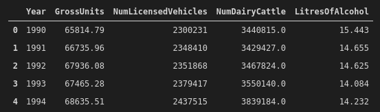
# what does it look like now?
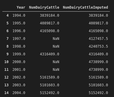
dat.head()

The most interesting thing we did here is to impute some missing values. From 1997 to 2001, four out of five years of cattle numbers data are missing. To address this, we imputed the values with a k-nearest neighbours method (from sklearn). I didn't overthink this (perhaps I underthought it), but in any case, the imputed data look okay:

And this is what the cleaned data look like now:

The last thing we want to do is to center the explanatory variables. There's actually some really interesting discussion on centering variables in regression models here (tl;dr is you can probably do it most of the time, but you also probably don't need to do it most of the time). We're going to YOLO it, and then we'll be good to go:

dat.NumLicensedVehicles = dat.NumLicensedVehicles - dat.NumLicensedVehicles.mean()
dat.NumDairyCattle = dat.NumDairyCattle - dat.NumDairyCattle.mean()
dat.NumSheep = dat.NumSheep - dat.NumSheep.mean()
dat.LitresOfAlcohol = dat.LitresOfAlcohol - dat.LitresOfAlcohol.mean()

Multiple regression

Like in part one, we're going to use the statsmodels.formula.api.ols function to construct our regression model. This time, however, we're going to add more than one explanatory variable. The syntax for this is pretty self-explanatory; we just add a plus sign followed by our extra variable for each one:

reg = smf.ols('GrossUnits ~ NumLicensedVehicles + LitresOfAlcohol + NumDairyCattle', data=dat).fit()

When we do this, we're effectively asking the question: "For each of the explanatory variables, is there a significant association with the gross amount of carbon dioxide emitted in New Zealand, if we account for the other variables?". In other words, for example, when we look to see whether the number of licensed vehicles is correlated with greenhouse gas emissions, we're holding litres of alcohol and number of dairy cattle constant in the model.

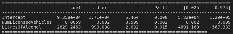
When we obtain a read-out of the model fit with reg.summary(), there are a few things to look at:

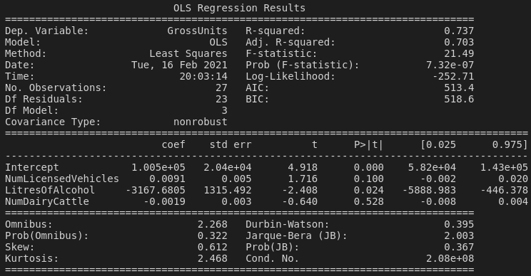
Our eyes are probably first going to fall on the coefficient table, and it's kind of funny. We can read the coefficient table in a similar way to how we interpreted the coefficients from our model with a single predictor variable. The only "statistically significant" correlation is with (millions of) litres of alcohol available for consumption in New Zealand (p = 0.024). Our coefficient here is negative, so this means that higher greenhouse gas emissions tend to be associated with lower availability of alcohol, and vice versa. An increase of 1 million litres of alcohol available for consumption is associated with a decrease in about 3000 CO₂-e units. Of course, we shouldn't ignore the huge standard error for this variable.

The other little thing to note is that, because we centered our explanatory variables, the intercept now represents the value of the response variable when the explanatory variables are held at their mean values. We can also look at the R-squared value and F-statistic, etc., but we talked about that last time. Let's go a bit further.

Hmmm...

If we were the curious type, we might think "hold on. Why should available alcohol be more strongly associated with greenhouse gas emissions than number of licensed vehicles? Surely the number of vehicles has a more plausible causal relationship?" And you know what's funny? If we run a univariate regression model, only taking into account the number of licensed vehicles, our resulting p-value is suddenly very low and we have a significant correlation:

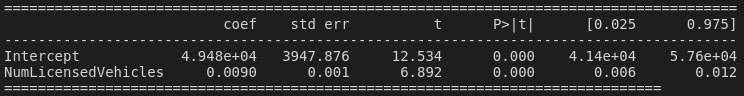
... and if we add LitresOfAlcohol back into the model, both variables have p-values for their t-statistics of less than 0.05!

So it appears that adding in NumDairyCattle has caused our best-guess explanatory variable, NumLicensedVehicles, to become non-significant!

Multicollinearity

We've just described that adding NumDairyCattle into our model caused the relationship between greenhouse gas emissions and the number of licensed vehicles in New Zealand to become non-significant. The reason for this is probably that those two explanatory variables are correlated with one another: we have multicollinearity.

This is a problem, because when we interpret coefficients in multivariate regression models, we're seeing how the response variable changes with the explanatory variable while we hold the other explanatory variables constant. When two variables are highly correlated, it becomes really difficult to test for the effect of one variable while holding the other one constant—because when one changes, the other changes with it! Yet again, I will link to a Statistics by Jim post on the subject, if you'd like further reading. In our case, however, one plausible approach is simply to remove one of the highly correlated variables.

Now, we can look at some more formal diagnostics!

Back to reality: evaluating model fit

There are a bunch of assumptions that we make when we fit a linear regression model. We should probably test those assumptions, right?

...right?

Q-Q plot

Guys, don't confuse your Q-Q and your P-P plots please.

In our context of regression, a Q-Q plot (for quantile–quantile) helps us address the assumption that our model's residuals are normally distributed. Remember that the residuals are just the errors of our model—how far away our predicted values of response variable are from the observed values. We plot the quantiles of the residuals estimated from the regression model against the quantiles calculated from a normal distribution. If the residuals follow a straight line (which we can add to the plot as reference), then they are normally distributed.

sm.qqplot(reg.resid, line='r')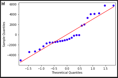

There isn't really a super black-and-white way of interpreting these, but to my inexperienced eye, the residuals don't seem to follow a straight line very well. I'm not sure that I'd be confident in saying that our assumption of normal distribution of residuals is validated!

Standard residual plot

We can construct a standard plot of the residuals of our model. I think this one is particularly revealing!

stdres = pd.DataFrame(reg.resid_pearson)
plt.plot(stdres, 'o', ls='None')
l = plt.axhline(y=0, color='r')
plt.ylabel('Standardized Residual')
plt.xlabel('Observation Number')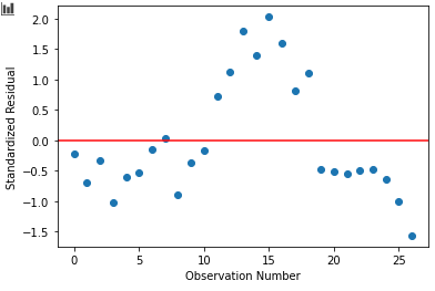

Because our model is linear—but the emissions aren't!—our residual plot is pretty awful. We're predicting emissions that are too high in the middle years, and too low in the early and late years. If you go back to the first post, you can see that the overall emissions took a bit of a dip between around 2007 to 2012. (Maybe because of the global financial crisis.) Our linear model is really struggling with this behaviour!

Leverage plot

The final metric we're going to use to evaluate our regression model is a leverage (or influence) plot. The residuals of our data are plotted against their leverage scores. These plots allow us to check whether any of our outliers are having a large effect on the model. It's useful to keep in mind that even if we do have "outliers" (however we want to define them), they might not actually change the model that much—so we might not need to worry about them.

sm.graphics.influence_plot(reg, size=8)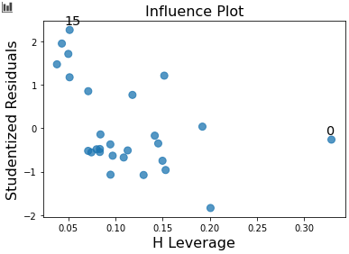

We're looking for values in the upper or lower right corners of the plot: these are observations with high effect on the model, so removing them is likely to change the resulting model coefficients much more significantly than removing other observations. In our case study here, we can't see anything too concerning, so there probably aren't many observations that are super influential on the model.

Conclusion

Well, that's it! If we were super confident, we might say something like "after accounting for the confounding effect of alcohol availability [lol], the number of licensed vehicles in New Zealand (beta = 0.0059, p = 0.002) is significantly and positively associated with New Zealand's gross greenhouse gas emissions". But in reality, we've made a fairly awful model that is riddled with problems. We've certainly violated the assumption of normality and linearity, and to be honest, I don't think we've really learned anything about greenhouse gas emissions. On the bright side, we've learned a lot about regression itself, and have taken a critical look at the model and managed to identify these issues with standard methodology like Q-Q plots and residual plots. Hopefully we'll be able to keep these things in mind the next time we feel a bit nerdy!

You can find all the code used in this post here.