Regression case study part one: New Zealand's greenhouse gas emissions

31 January, 2021

Check out part two here.

Introduction

This is the first of two posts describing the development and evaluation of a regression model in Python. In this first section, I'll describe the data itself—data on New Zealand's greenhouse gas emissions from 1990 to 2016—and in the second section, we'll look at how to construct a simple linear regression model. The second post in this series delves into multiple regression, and more advanced ways to evaluate model fit and specification.

Part one: the data

Sample

This project uses the New Zealand’s greenhouse gas emissions 1990–2016 dataset. The data were sourced from the Greenhouse Gas Inventory of New Zealand's Ministry for the Environment (MfE), and were released as part of MfE's Environment Aotearoa 2019 report. The Greenhouse Gas Inventory is produced by MfE every year, and forms part of New Zealand's reporting obligations under the United Nations Framework Convention on Climate Change and the Kyoto Protocol.

The dataset contains measurements of gases added to the atmosphere by human activities in New Zealand—that is, excluding natural sources of greenhouse gases, such as volcanic emissions and biological processes—from 1990 to 2016. The data were aggregated into sector-specific categories, and comprise 306 distinct numerical measurements of greenhouse gas emissions, spread across 17 years and five main sectors. The entire dataset is used for this project.

Procedure

The data were obtained experimentally, by measuring the amount of greenhouse gas emissions that different sectors in New Zealand produce. The data were collected from 1990 to 2016, across New Zealand and by different reporting bodies.

While MfE compiles the Greenhouse Gas Inventory, the responsibility for reporting greenhouse gas emissions falls upon different government agencies, according to sector:

The Ministry for the Environment reports on industrial processes and other product use, waste and land use and forestry;
Energy emissions are reported by the Ministry of Business, Innovation and Employment;
and Agriculture emissions are reported by the Ministry for Primary Industries.

Finally, MfE provide further guidance on the measurement and reporting of greenhouse gas emissions in New Zealand.

Measures

The dataset comprises four variables:

Gas (type of gas emitted; categorical variable with primary levels of CO₂ (carbon dioxide), CH₄ (methane) and N₂O (nitrogen dioxide). The sum of the measured gases by sector was also reported as All gases.
Source (source of gas emissions by sector). Emissions were grouped into five major sectors according to the process that generates the emissions. The sectors are Agriculture, Energy, Industrial processes, Waste and Land use;
Year (1990 to 2016);
and carbon dioxide equivalent units.

The data were obtained in a wide format with the "Year" variable spread across columns. The numerical measure of greenhouse gas emissions is expressed in carbon dioxide equivalent (CO₂-e) units, which measures how much global warming a given type and amount of greenhouse gas causes. This is used to enable us to compare the effect of different types of greenhouse gas in a consistent way, so that we can compare the relative contribution of different gases to the greenhouse effect, regardless of the actual amounts emitted. The values ranged from less than –30,000 CO₂-e to over 80,000 CO₂-e units. Negative values of CO₂-e were attributed to the Land use sector due to the carbon sequestration effects of forestry. The emission sector and the year were treated as potential explanatory variables, while the CO₂-e unit values were treated as the response variable.

Part two: simple regression

First steps with Python

Before we construct our model, let's have a quick look at the data, which were downloaded on 2 February 2020.

import pandas as pd
import seaborn as sns
import statsmodels.formula.api as smf

dat = (
    pd.read_csv('data/new-zealands-greenhouse-gas-emissions-19902016.csv')
        .melt(id_vars=['Gas','Source'],
            var_name='Year', value_name='Units')
        .astype({
            'Year': 'int32',
            'Gas': 'category',
            'Source': 'category'    
        })
)

dat.head(6)

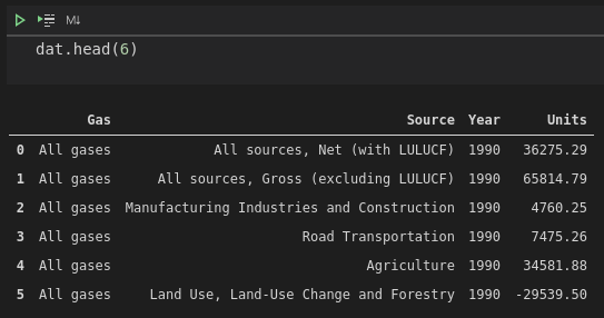
We've used pandas.melt to pivot the data to a long format, giving us Gas, Source and Year explanatory variables. Our Units variable contains the measured CO₂-e units for each observation.

One thing you might notice straight away is that there is a negative number in the Units field. This occurs when Source is equal to "Land use, land-use change and forestry". Also known by its abbreviation of LULUCF, this category represents both emissions and removal of emissions from the atmosphere due to land-use changes. In New Zealand, for this period, the values are negative, indicating that LULUCF was a net remover of greenhouse gas emissions, rather than producer.

Keeping that in mind, I thought it'd be a good idea to whip up a quick plot showing the change of net greenhouse gas emissions (i.e., including LULUCF and the role of forestry in removing emissions from the atmosphere) compared to gross greenhouse gas emissions (ignoring removal) over the period of the data we have available:

summary = dat.query("Gas == 'All gases' & Source.isin(['All sources, Net (with LULUCF)', 'All sources, Gross (excluding LULUCF)'])")
summary.Source = summary.Source.cat.remove_unused_categories()
sns.lineplot(data=summary, x='Year', y='Units', hue='Source')

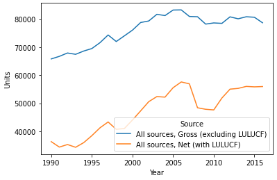
It's clear that LULUCF really does play an important role in mediating New Zealand's greenhouse gas emissions. But back to the point of this post, which is to demonstrate simple regression with Python—let's construct a model that uses Year as the explanatory variable, and net emissions as the response variable. Basically, we'll see if that trend that we see with our own two eyes—emissions increasing over time—is statistically significant in a linear regression model.

I should add at this point that, of course, Year is absolutely not a real explanatory variable. Arbitrarily changing the year shouldn't change anything about greenhouse gas emissions. Instead, Year will be correlated with the true explanatory variables, like increases in number of cars on the road, increases in number of dairy farms, etc.

The model

Actually creating a simple linear regression model is really straightforward. We use the statsmodels.formula.api function ols (for ordinary least-squares), and fit the model on the data for net greenhouse gas emission units:

net_summary = summary[summary.Source == "All sources, Net (with LULUCF)"]
reg = smf.ols('Units ~ Year', data=net_summary).fit()

Printing the output of the model gives us a bunch of useful (and at first confusing) information:

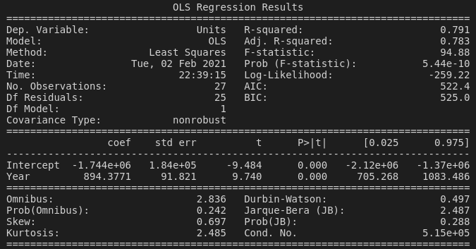
Model and Method remind us that we've made an ordinary least-squares model.
The R-squared value of 0.791 tells us that about 79% of the variance in greenhouse gases can be explained by the Year variable. (Let's be careful here again -- Year doesn't actually have any real relationship with greenhouse gas emissions, it's completely arbitrary, right?)
The F-statistic of 94.88 tells us that our model, taking into account the Year variable, fits better than a model with only the intercept (i.e., no explanatory variables). I'm going to defer to Jim's explanation of the F-statistic in the context of regression models here, if you'd like a more in-depth explanation.
The Prob (F-statistic) value of 5.44 x 10 tells us that our F-statistic is almost certainly not so high by chance, and therefore that our model (showing Year as a good predictor of greenhouse gas emissions) is statistically significant.

Underneath these statistics is the coefficient table, with two entries: Intercept and Year.

The coef (coefficient) of 894 for the Year variable tells us that each year tends to see an increase in greenhouse gas emissions of about 894 units. This is important because the whole point of running this regression analysis is to see whether the coefficient of our explanatory variable(s) is different from zero—i.e., has an effect on the response variable—and of course, whether this difference is due to chance or not.
The t-statistic is simply the coefficient divided by the standard error. I personally find it difficult to interpret the t-statistic in a regression context, particularly coming from a background of using t-tests to compare two population means. There is a very math-heavy explanation here, and quite a good overview of all the outputs of a regression model, including the t-statistic, here. However, just looking at its definition—the coefficient divided by the standard error—we can maybe think intuitively here. If the standard error is nearly as large as the coefficient, then the coefficient probably isn't going to be that useful, as the explanatory variable (Year for us) isn't going to be able to predict the response variable without a large amount of error. But really, we can skip over all this and just look at the p-value:
The P>|t| value of 0.000 (or, I suppose, less than 0.001) tells us that the t-statistic is statistically significant (there is a less than 0.1% chance that we would have collected these data if the null hypothesis were true, that Year has no effect on greenhouse gas emissions).
Finally, we can see the two-tailed 95% confidence interval values for the coefficient ([0.025 and 0.975, respectively).

And that's basically it for our first model. Our fit suggests that Year is a pretty good predictor of net greenhouse gas emissions, with emissions tending to increase by between around 700 to 1100 CO2-_e units per year!

Next, we're going to look at multiple regression and evaluating model fit.

You can find all the code used in this post here.