Simple chi-squared test with Python

21 January, 2021

Introduction

We can use the chi-squared test when we want to know whether one categorical variable is correlated with another categorical variable. For example, whether the size of a car's engine (in terms of number of cylinders; our categorical explanatory variable) predicts the car's fuel efficiency in miles per gallon (our categorical response variable). We'll show how to do this in Python.

Note: If you instead want to understand how a categorical explanatory variable affects a quantitative (or continuous) response variable (like, how the species of plant affects the plant's leaf measurements), check out this previous post, where we use the ANOVA statistical test instead.

Setting up

To get started, we'll be importing a few important libraries. We'll be using the mpg dataset, which seaborn conveniently makes available to us as a pandas data frame. The mpg dataset gives the miles per gallon (mpg) of a few hundred cars, along with some characteristics of the cars, like the number of cylinders that make up the engine, the horsepower, weight, and so on.

import pandas as pd
import numpy as np
import scipy.stats
import seaborn
import matplotlib.pyplot as plt

mpg = seaborn.load_dataset('mpg')

Since the chi-squared test needs two categorical variables, we're going to convert the mpg variable into a grouped category. We'll split mpg into four different groups: those cars with mpg between 10 and 19; those with mpg between 20 and 29; 30 to 39 and 40 to 49. We'll keep the raw mpg as reference.


# only take observations where cyl is either 4, 6 or 8
mpg = mpg[mpg['cylinders'].isin([4,6,8])]
# convert to categorical variable
mpg['cylinders'] = mpg['cylinders'].astype("category")

# categorise into 10-mpg ranges
labels = ["{0} - {1}".format(i, i + 9) for i in range(10, 50, 10)]
mpg['mpg_group'] = pd.cut(mpg.mpg, range(10, 60, 10), right=False, labels=labels)

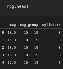
This is what the first few rows of our new dataset look like:

How it actually works

The chi-squared test operates on a contingency table. This is where we group our observations into categories, and count the number that fall into each combination of variables. In our example, that means looking at the dataset and finding all cars with four cylinders. Of those cars, we then count how many were in the 10–19 mpg group, how many were in the 20–29 mpg group, and so on. Then, we move onto cars with six cylinders; of those, we count how many were in each mpg group. We end up with a contingency table that shows the frequencies of observations in each combination of variables. We can use the pandas function crosstab to generate our contingency table:

contingency_tbl = pd.crosstab(mpg['mpg_group'], mpg['cylinders'])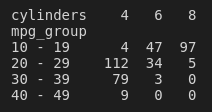

Our hypothetical explanatory variable lies along the top row. We are thinking that the number of cylinders might affect the fuel efficiency in mpg of the cars in the dataset. Looking at our table, for cars with a fuel efficiency of between 20 and 29, 112 of them have four cylinders. Only 34 are six-cylinder cars, and a measly five are eight-cylinder cars. Maybe we're onto something here.

The next thing that the chi-squared test does is calculate the frequencies that would be expected if there were no relationship between number of cylinders and miles per gallon. That's the null hypothesis. We could say that the null hypothesis states that the number of cylinders in a car's engine has no effect on the fuel efficiency of that car. Then, the chi-squared test measures how far away the observed data are from the expected data. If the observed data are very far away from the expected data, then we reject the null hypothesis.

Another way to look at it is by looking at percentages, rather than counts. To do this, we'll divide the counts in the contingency table by the column sums:

contingency_tbl/contingency_tbl.sum(axis=0)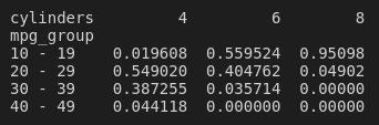

The percentages in each column sum to 100. So, for example, we can see that, of the cars with 8 cylinders, approximately 95% of them have a fuel efficiency of 10 to 19 mpg! Conversely, only about 2% of the cars with four cylinders have a fuel efficiency that low.

Doing the thing

Anyway, we're now ready to run the actual chi-squared test on the contingency table. It's pretty simple:

scipy.stats.chi2_contingency(contingency_tbl)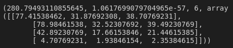

Alright, the output looks pretty confusing, but we're only really interested in the first two numbers. The first number, 280.79, is the chi-squared statistic. The higher the number, the larger the relationship between the explanatory and response variables. A number this high means a pretty good relationship! The second number, 1.06e-57, is the p-value. This is small, so this chi-squared result is almost certainly not just by chance. Great!

Of course, we always want to draw some nice plots, and we should probably check that the data actually agrees with our statistical conclusions! So we can make a plot that shows the effect of cylinder number on fuel efficiency, using the means of the raw mpg numbers from the original dataset:

mpg.groupby('cylinders').mean()['mpg'].plot(
    kind='bar',
    xlabel='Number of cylinders',
    ylabel='Mean miles per gallon')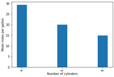

Yep—looks like the cylinders do have an effect on the fuel efficiency! (Okay, we've totally just done this completely back-to-front: we would normally find something like this when we're doing our exploratory data analysis and making a bunch of plots, hoping to see some interesting relationship between variables. After we've discovered something like this, then we go and do some stats to check whether the relationship is significant or not. But sue me.)

Hold on...

We have a high chi-squared statistic and a very low p-value, so there is a statistically significant relationship between the number of cylinders and the fuel efficiency of cars. But is that true for all different levels of cylinders? That is, are cars with four cylinders more fuel efficient that those with six? Or is it just cars with eight cylinders that are more fuel efficient than those with four? Our single chi-squared statistic can't actually tell us this.

In my previous post on ANOVA, I talked a little bit about why we can't just compare each category separately without applying some sort of correction to account for the family-wise error rate. For that case, we used Tukey's correction. Here, however, we're going to make use of the Bonferroni correction to account for the effect of multiple comparisons on the chance of coming up with a false positive. With this technique, we simply divide the desired p-value (say, 0.05) by the number of comparisons being made. In this case, we just have three comparisons: four and six cylinders, four and eight cylinders, and six and eight cylinders. Therefore, our adjusted p-value is 0.05 / 3 = 0.017. This means that we'll only consider a comparison statistically significant if the p-value is less than 0.017 (rather than less than 0.05).

Finally, we're just going to create a list of combinations to loop over. For each iteration of the loop, we'll subset the data to only include that particular combination of cylinders, and create a contingency table using that data. Then, we'll run the chi-squared test on the contingency table, comparing just two levels of the cylinder variable at a time.

combns = [
    [4, 6],
    [4, 8],
    [6, 8]
]

for i in combns:
    this_subset = mpg[mpg['cylinders'].isin(i)]
    contingency_tbl = pd.crosstab(this_subset['mpg_group'], this_subset['cylinders'])
    print('Comparing ' + str(i))
    print(scipy.stats.chi2_contingency(contingency_tbl))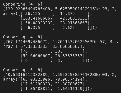

A quick glance over the results shows that, for each of the comparisons, the chi-squared statistic was high and the p-value was less than 0.017—we've found that cars with four-cylinder engines have statistically significantly higher fuel efficiency than those with six- or eight-cylinder engines, and cars with six-cylinder engines also have statistically significantly higher fuel efficiency than those with eight-cylinder engines!

At this point, we try not to think about the fact that we intuitively knew that already...

You can find all the code used in this post here.