Simple ANOVA with Python

20 January, 2021

Introduction

We can use analysis of variance (ANOVA) to check whether the means of two or more groups in a sample are equal. If you have a categorical explanatory variable and a continuous response variable, ANOVA is probably a good choice to try to answer whether the explanatory variable does, in fact, explain the differences in the response variable.

For example, say we go out and collect a bunch of leaves from three different species of plant, and then carefully measure the length and width of them. (Okay, we "pay" a student to do this for us, and hope that they know how to use a ruler.) We hypothesise that the type of species will be correlated to the length and width of the leaves. In this case, species is an explanatory (or predictor) variable, because we think it's going to explain the measurements of the leaves; and the measurements of the leaves are our response (or outcome) variables, because we think they will respond to, or be predicted by, the species.

In this brief note, we'll show how to set up and run a simple ANOVA test on our dataset, to see whether we were right or not—whether species actually does predict the length and width of leaves. For this task, we'll use Python.

Prerequisites

I'm using Python 3.8.6, but probably any version of Python 3 will be fine. If you haven't already, install pandas, statsmodels and seaborn from the terminal:

pip install pandas
pip install statsmodels
pip install sklearn

pandas probably needs no introduction, and we're using the data visualisation libraryseaborn because it has conveniently packaged up a version of the iris dataset for us as a pandas data frame. statsmodels provides us with the actual functions used to run the ANOVA.

Doing the thing

Firstly, we import the libraries that we need, and load the iris dataset:

import pandas as pd
from seaborn import load_dataset
import statsmodels.formula.api as sm
import statsmodels.stats.multicomp as multi

iris = load_dataset("iris")

If you're familiar with the dataset, you'll know it has four continuous variables describing the petal and sepal length and width, and one categorical variable. The categorical variable, species, has three levels (or groups): setosa, versicolor and virginica.

The simplest way of conducting an ANOVA test is with a dataset whose categorical explanatory variable contains only two levels. Typical examples of this could be sex (male or female), or something like a yes-or-no answer, like "do you smoke?". To run our first ANOVA in this way, we'll subset the iris dataset to only include the setosa and versicolor species:

my_subset = iris[iris["species"].isin(['setosa', 'virginica'])]

We're actually ready to run our model now! We pass in our model formula to the ols function in the statsmodels library. We can interpret our formula syntax sort of like this, with a tilde in the middle:

'<response variable> ~ <explanatory variable>'

Or, "...test what effect our explanatory variable has on our response variable." We wrap the explanatory variable up in C(...), which just says that it's a categorical variable. Finally, we print out the summary of the model's fit:

subset_model = sm.ols(formula='sepal_length ~ C(species)', data=my_subset)
subset_model.fit().summary()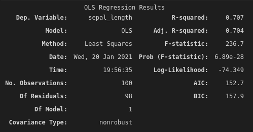

Interpretation

F-statistic

The summary of the model's fit contains quite a lot of information! But we'll just focus on a couple of important statistics. The first is the F-statistic. In this case, we have an F-statistic of 236.7. That's pretty high! But what does it mean?

The F-statistic is the ratio of the variance of the sample group means over the variance within the sample groups. That's a bit abstract, though. What it's really telling us is to what extent does the variation between group means dominate over the variation within the groups themselves. A high F-statistic means that the variance between the groups is greater than the variance within the groups. In other words, the groups are probably different!

So we've looked at our F-statistic of 236.7, and said to ourselves, "okay, the measured sepal lengths of the setosa species seem quite different to the measured sepal lengths of the versicolor species." Now, we need to see whether this is a significant correlation or not. For that, of course, we look at the p-value.

p-value

In the output from this model, we can find our p-value listed as "Prob (F-statistic): 6.89e-28". Wow, okay, that's a really small number. It's outside of the scope of this post to talk about p-values, but they're effectively saying, "if the null hypothesis were true, how likely is it that a random sample of the population would give us this data?". In our case, this extremely low p-value is telling us that it's really unlikely that we'd have collected this data, if the sepal length of setosa and versicolor leaves are actually the same (ignoring how poor our student is with a ruler). So, we're pretty happy that the sepal lengths are significantly different!

Sense-check

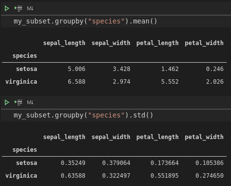
my_subset.groupby("species").mean()
my_subset.groupby("species").std()

It's always a good idea to make sure that our interpretation of the model isn't totally wrong. If we quickly check the mean and standard deviation of our iris data after grouping by species, we can see that the mean sepal length for setosa is about 5, compared to about 6.6 for versicolor. The standard deviations are about 0.4 and 0.6, respectively. At this point, we can be pretty happy that we've found a real relationship between species and sepal length.

What about the other species?

Remember how we subsetted the iris dataset to only include two species? If we want to compare more than two levels of a categorical variable, we'll have to run a post-hoc (after the fact) test on our model. You could be thinking, "Why don't we just run ANOVA on species 1 vs species 2; then on species 1 vs species 3; then on species 2 vs species 3?" Well, the more tests that we run, the higher our chance of finding a false positive, or a type 1 error, where we erroneously reject the null hypothesis. Remember our really low p-value? Well, imagine that it actually came back as 0.05. One way of interpreting that value is that, if there were no difference in the sepal lengths between the two species, then we'd get the data that we collected about five percent of the time. We have a five percent chance of making a mistake in our assertions.

The more tests that we run, the higher our chance of coming up with false positives. In another life, I used to extract metabolites from things like milk and grass, and run them through mass spectrometers, to try to find differences in the abundance of the metabolites across different groups in the dataset. (Maybe this type of grass has higher levels of this sugar than that type of grass.) The thing is, we would end up with hundreds if not thousands of metabolites to go through. If we used a raw p-value, we would end up with dozens and dozens of false positives; so we needed to take into account the false discovery rate when calculating the p-values. This is a similar idea to the family-wise error rate. The more comparisons you make, the higher your chances of a false positive!

So, what do we do about it? Well, there are several methods used to address this issue, which give us p-values that are a bit more strict, and less likely to be false positives. One of these methods is the amusingly named Tukey's honestly significant difference (HSD) test. To run this test, we'll be using statsmodels.stats.multicomp.MultiComparison. We'll simply pass it the sepal length and species vectors from the original iris dataset, and grab the summary of the Tukey's HSD test:

multi_comp = multi.MultiComparison(iris['sepal_length'], iris['species'])
multi_comp.tukeyhsd().summary()

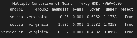
Each row of the summary output is a single comparison between two groups. Most of the things in this summary are pretty easy to understand on the surface: we have the difference in means between groups, the adjusted p-value (adjusted using Tukey's HSD method), lower and upper confidence, and the most succinct summary: reject. If reject is True, then we reject the null hypothesis that the group means are equal. In other words, we accept the alternative hypothesis, that the group means are different.

You can find all the code used in this post here.