Training vs test mean squared error in R
Introduction
The mean squared error (MSE) is the mean of a model's residuals. When you fit a regression model predicting some continuous response variable, and then use that model to predict the values of some data, the residuals are the differences between the values that your model predicts, and the actual values in the data. Residuals and errors are the same thing in this context.
I grabbed some data from Kaggle and fit a simple regression model that predicts the happiness level of a country based on a bunch of things like GDP and level of social support. I then used that model to predict the happiness level of some new countries that weren't included in the model, and here's a residual plot of that data:
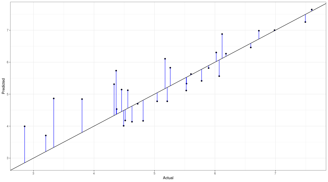
Each point on the plot is a different country; the actual happiness score for that country is on the x-axis, and the predicted happiness score is on the y-axis. The black line going through the middle is where the actual and predicted values converge. If our model was perfect, then every point would lie along that line. Of course, even if our model predicted the actual coefficients perfectly, there's always going to be some random error that can't be accounted for, so we'll always get some level of error. I added some blue vertical lines to the plot showing the distance from each predicted point to the actual value. A longer line means greater error.
So, those lines represent the residuals. To calculate the MSE, we need to square the residuals, so that a negative residual has the same contribution to the mean as an equivalent-magnitude positive residual. For example, say the actual value of the response variable was 7, and we predicted 5. The residual is 5 – 7 = –2. By squaring that residual, it would end up being the same as a residual that resulted from a prediction of 9, since 9 – 7 = 2, and 22 is the same as –22. Anyway, we calculate all the residuals, square them all, take the mean, and voila: that's our MSE.
I trained the model on a subset of countries, and then used a different subset of countries to evaluate the fit of the model. Therefore, if we were to calculate an MSE based on the data in the plot above, that would be a test MSE. Awesome. So what's a training MSE? And why do we need to care?
Training MSE
Let's use the diamonds dataset in the ggplot2 package to explore this.
library(ggplot2)
library(dplyr)
We'll train a simple linear regression model, predicting the price of a diamond based on carat (that's its weight). We use data = diamonds, because we're using the entire dataset to fit the model:
train_mod <- lm(price ~ carat, data = diamonds)Then, we use the model to predict the values of price (yep, we're predicting on the same observations that we trained the model with):
y_hat_train <- predict(train_mod, data = diamonds)y_hat_train is a numeric vector containing the predicted values of price for each observation in the diamonds dataset. Now that we have these predicted values, we can calculate the training MSE. It's the training (rather than the test) MSE because we haven't split our dataset into training and test sets; instead, we fit our model on the entire dataset, and now we're evaluating it on the same dataset.
So, we calculate the training MSE by getting the residuals, squaring them, and taking the mean:
train_MSE <- mean((diamonds$price - y_hat_train)^2)This is basically what the model will be doing, where the blue line is the predicted value:
ggplot(diamonds, aes(x = carat, y = price)) +
    geom_point() +
    geom_smooth(method = "lm") +
    scale_y_continuous(limits = c(0, 20000))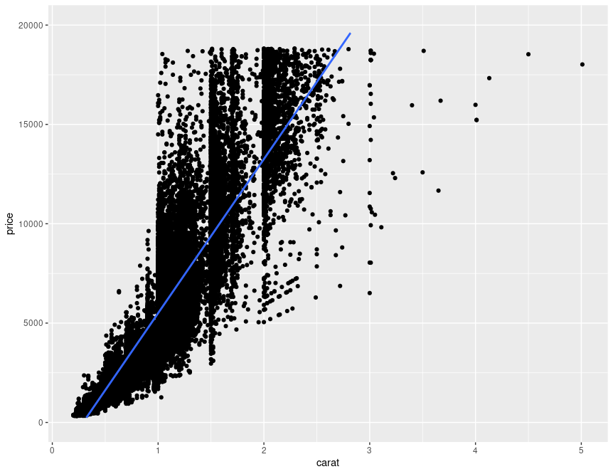
There's some significant nonlinearity in the relationship between price and carat that isn't captured by our simple model (which only includes linear terms). Our model therefore isn't providing a great fit to the data, and the training MSE is probably going to be quite high.
So how about we fit a series of polynomial models that may be able to capture that nonlinear relationship better? (A log transformation would probably be more appropriate, but bear with me...) We'll construct ten models, with one- to ten-degree polynomials of carat. That is, our first model will be a first-degree polynomial (er, it'll just be our linear model); the second one will have a second-degree polynomial, so there will be terms for carat as well as carat2; and so on, until we fit a model with a tenth-degree polynomial.
training_mses <- list()
for (i in 1:10) {
    train_mod <- lm(price ~ poly(carat, degree = i), data = diamonds)
    train_y_hat <- predict(train_mod, data = diamonds)
    training_mses[[i]] <- mean((diamonds$price - train_y_hat)^2)
}
As we can see, adding higher-order polynomials tends to decrease the training MSE:
tibble(
    polynomial = 1:10,
    MSE = unlist(training_mses)
) %>%
    ggplot(aes(x = polynomial, y = MSE)) +
        geom_line(aes(group = 1)) +
        scale_x_continuous(breaks = 1:10)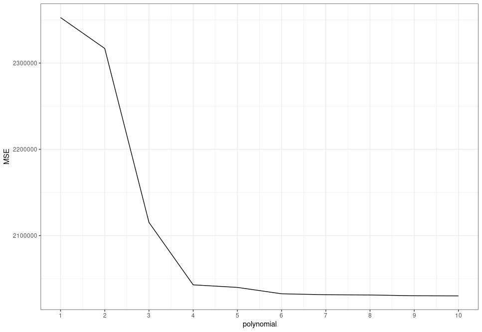
So what's the issue with these higher-order polynomials? They give us models with lower errors, right?
We'll, we're overfitting the model! Adding those higher-order polynomials made our model great at predicting data it has already seen, but it'll probably not be so great at predicting brand new data. Those higher-order-polynomial models will have high variance (meaning, they won't be very accurate). So if we were just basing our model-picking decisions on training MSE, we would very quickly end up with a model that performs poorly in the real world. We need to use test MSE, instead.
Training vs test MSE
Let's see what happens when we split the data into training and test sets, and evaluate test MSEs instead of training MSEs. We'll sample 70% of the data for the training set, leaving 30% for the test set.
set.seed(1)
dat <- list()
dat[['index']] <- sample(nrow(diamonds), size = nrow(diamonds) * 0.7)
dat[['training']] <- diamonds[dat$index, ]
dat[['test']] <- diamonds[-dat$index,]
Now let's fit our ten models against the training set, but calculate test MSEs as well as training MSEs.
Note that we must specify newdata = dat$test, to make sure we're predicting the test set price values!
test_mses <- training_mses <- list()
for (i in 1:10) {
    train_mod <- lm(price ~ poly(carat, degree = i), data = dat$training)

    y_hat_training <- predict(train_mod)
    training_mses[[i]] <- mean((dat$training$price - y_hat_training)^2)

    y_hat_test <- predict(train_mod, newdata = dat$test)
    test_mses[[i]] <- mean((dat$test$price - y_hat_test)^2)
}
Now when we look at the test MSE, we can see that it isn't as simple as just maxing out the polynomials—there isn't a clear pattern of higher-degree polynomials leading to lower MSEs:
tibble(
    polynomial = rep(1:10, times = 2),
    MSE = c(unlist(training_mses), unlist(test_mses)),
    Type = rep(c("Training", "Test"), each = 10)
) %>%
    ggplot(aes(x = polynomial, y = MSE, colour = Type)) +
        geom_line(aes(group = Type)) +
        scale_x_continuous(breaks = 1:10) +
        theme_bw()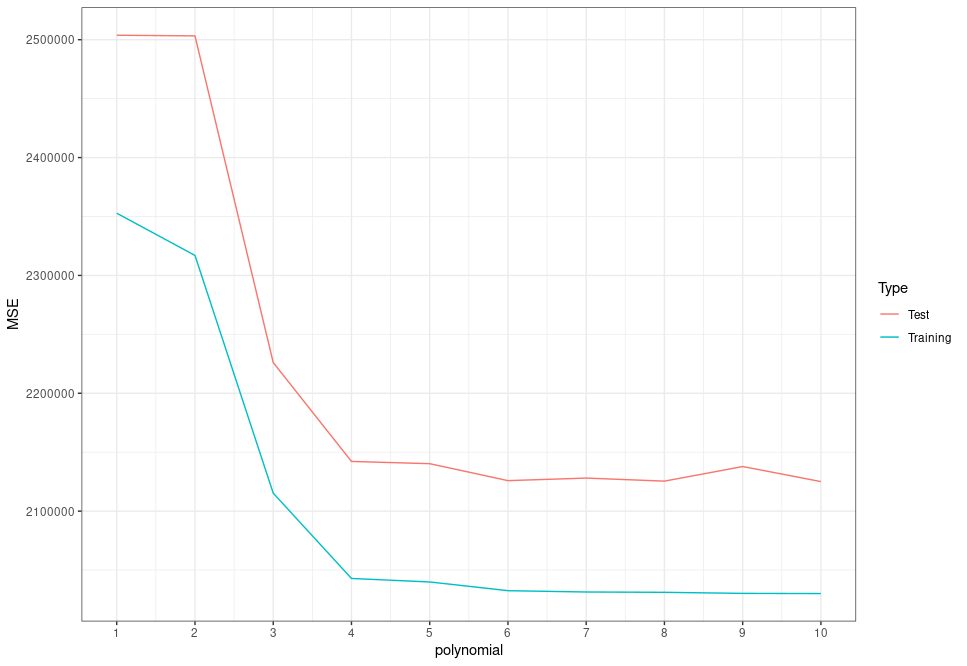
While the training MSE continues to fall with increasing polynomial order, the test MSE doesn't. In fact, the model with a ninth-degree polynomial for carat actually has higher error than those with sixth-, seventh-, eighth- and tenth-degree polynomials! The extra complexity of the higher-order polynomials allowed the regression coefficients to be estimated very precisely; almost too precisely. We started picking up on patterns in the data that weren't really there, or at least were only there in the training set, and not in the test set (and presumably not in the general population). This extra complexity made our models great at predicting values it had already seen before, but not so great at predicting new data. This is overfitting, and it's why we should use the test MSE to evaluate our models, rather than training MSE!
Umm, so which model should we actually choose?
It looks like the test error falls significantly as we increase model complexity up to the fourth-degree polynomial. After that, it falls and rises by relatively small amounts as we fit successively higher-order-polynomial models. The fourth-degree polynomial model certainly doesn't have the lowest test MSE; that's probably the sixth- or eighth- or tenth-degree model. However, we shouldn't necessarily always go for the model with the lowest MSE; we want to balance model performance with model complexity, as well as keeping in mind that a particular test MSE isn't necessarily statistically significantly lower than a similar one. So, we use the one-standard-error rule.
This rule states that we should choose the simplest model with a test MSE within one standard error of the best model. There's a really good breakdown of this rule here. Briefly, let's find the model with the lowest test MSE:
which.min(unlist(test_mses))
## [1] 10
Alright, the model with the tenth-degree polynomial had the lowest test MSE. Now we calculate the root mean squared error (RMSE) for this:
best_RMSE <- sqrt(test_mses[[10]])
best_RMSE
## [1] 1457.761
Adding the RMSE to the best test MSE, we get an upper-limit test MSE for a candidate model of:
test_MSE_limit <- best_RMSE + test_mses[[10]]
test_MSE_limit
## [1] 2126524
And finally, which is the simplest model with a test MSE within the upper limit of 2126524?
which(unlist(test_mses) < test_MSE_limit)[1]
## [1] 6
We therefore choose model with the sixth-degree polynomial! The porridge isn't too hot; it's not too cold, either; this porridge is just right. (Theoretically.)
References
- This one's a bit awkward; I based this post on things I learned from DATA473 - Statistical Modelling for Data Science, a course at Victoria University of Wellington. Dr Yuichi Hirose was the lecturer that talked about training vs test MSE; so, thanks Yuichi :)
- Cross Validated - Empirical justification for the one standard error rule when using cross-validation