The inverse-transform method for generating random variables in R
You can find all code used in the blog post here.
Introduction
This post describes how to implement the inverse-transform method for various distributions in R. The inverse-transform method is a technique of generating random variables from a particular distribution. It relies on a clever manipulation of the cumulative distribution function (CDF). Let's start there.
The CDF of a random variable \(X\) evaluated at \(x\) is the probability that \(X\) will take a value less-than or equal to \(x\). Okay, what does that mean? Well, here's the CDF of a normal distribution with \(\mu = 0\) and \(\sigma = 1\):
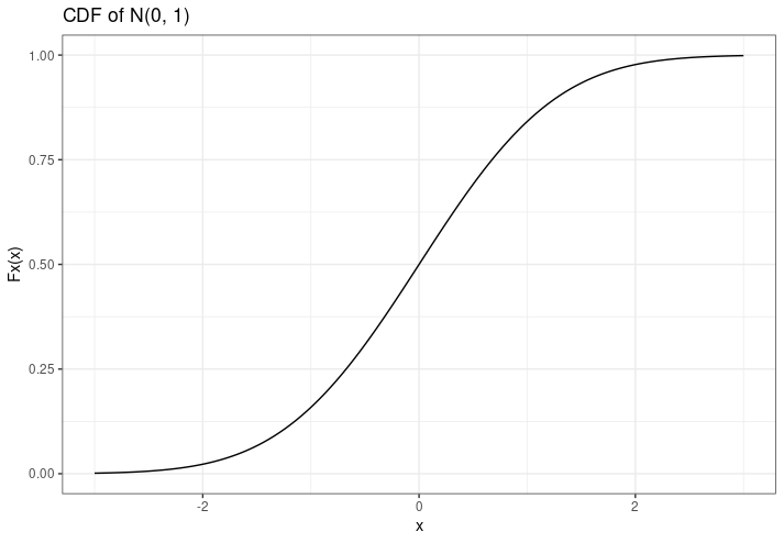
The CDF is often represented by \(F_X(x)\), and is shown on the y-axis. Let's use an example to see what it means. Say we sample one random variable from this normal distribution (with a mean of 0 and a standard deviation of 1), and we get a value of \(x = 0.3\). We read the CDF by looking at the x-axis, tracing directly up from our value until we hit the CDF line, and then going left to find the value on the y-axis. It might look like this:
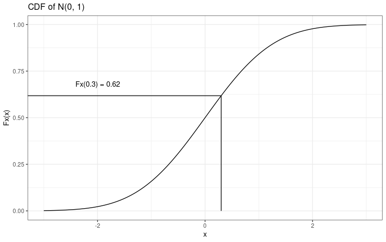
I promise I'm not just mansplaining how to read a simple x–y graph; I'll explain where I'm going this with in a moment. Anyway, in R, we can use the pnorm function to evaluate the CDF of a normal distribution, e.g.,
x_val <- 0.3
y_val <- pnorm(x_val)
y_val
# [1] 0.6179114
So what does it mean? Well, it means that when you draw a random sample \(x\) from that distribution, there's about a 62% chance that \(x \leq 0.3\). The CDF is a probability, so it ranges from 0 to 1. People smarter than me say it's a "monotonic increasing" function, meaning that it only ever increases as x-values increase. It's cumulative, right? So it only increases. Okay.
And now we get to the main idea of the inverse-transform method. Instead of evaluating the CDF at \(x\), we evaluate the inverse CDF at \(u\), where \(u\) is a random variable from a uniform(0, 1) distribution. This is basically the reverse of what we've just done: We start with a value between 0 and 1 (on the y-axis), and use the inverse CDF to convert that into an appropriate x-value for that particular distribution. \(x\) becomes a function of \(y\), not the other way around.
By the way, this is what 1000 random samples from a uniform(0, 1) distribution looks like—1000 values distributed randomly between zero and one:
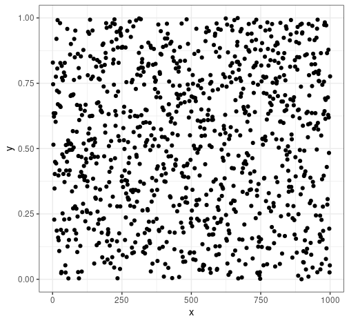
That's why we use a uniform(0, 1) distribution—it simulates the possible values of a CDF.
Side note: If you don't know the CDF, you can express is as the integral of the PDF \(f(x)\) from \(0\) to \(x\),
$$ F_X(x) = \int_0^xf(t)dt. $$
So if you can figure out how to integrate your particular probability distribution (have fun), then you can obtain the CDF and go from there. Or just, like, look it up on the internet.
Sampling from a continuous distribution
We can describe a simple algorithm describing the inverse-transform method for generating random variables from a continuous distribution as follows:
- Step 1: Generate \(u\) from uniform(0, 1);
- Step 2: Return \(x = F_X^{-1}(u)\).
The first step is trivial (in R, we'll use runif). The hard part is probably going to be finding an expression for the inverse CDF, \(F_X^{-1}\). In practice, this means setting the CDF of the relevant distribution equal to \(u\), and then solving for \(x\). The best way to demonstrate this is with lots of examples, so here goes!
Kumaraswamy distribution
Let's assume we've endured a fun journey through calculus, and have found that the CDF of a Kumaraswamy distribution can be expressed as \(F_X(x) = 1 - (1 - x^a)^b\) (or maybe we just looked it up). We now set that equal to \(u\) (our uniform random variable), and solve for \(x\):
$$ \begin{aligned} u &= F_X(x) \\ &= 1 - (1 - x^a)^b. \\ \end{aligned} $$ $$ \begin{aligned} &\implies 1 - u = (1 - x^a)^b \\ &\implies(1 - u)^{1/b} = 1 - x^a \\ &\implies1 - (1 - u)^{1/b} = x^a \\ &\implies x = (1 - (1 - u)^{1/b})^{1/a}. \end{aligned} $$
Now that we have the inverse CDF, we can implement the inverse transform method. We set the parameters \(a\) and \(b\), and generate 10,000 random values from the uniform distribution in the vector \(u\):
# set parameters
a <- 1/2
b <- 2

# generate 10,000 random uniform variables
set.seed(1)
u <- runif(10000)
We then evaluate the inverse CDF to generate 10,000 random values from the Kumaraswamy distribution. This part requires us to write the inverse CDF as R code, like this:
generated_vals <- (1 - (1 - u)^(1/b) ) ^(1/a)And that's it! We've generated 10,000 random variables using the inverse-transform method. What more is there to look forward to in life?
Well, one more thing to look forward to is having excuses to draw pretty plots. To verify that our generated values actually make sense, we can construct a histogram of them, which should resemble the theoretical PDF. So, if we do that, and plot it alongside the theoretical PDF generated from a sequence of \(x\) values in R, we get this:
# get the exact values of the PDF
x <- seq(0.01, 1, length.out = 10000)
theoretical_pdf <- a * b * x^(a-1) * (1 - x^a)^(b-1)

# create list to hold our two plots
plts <- list()

# constuct histogram of generated values
plts[[1]] <- tibble(generated_vals = generated_vals) %>%
    ggplot() +
        geom_histogram(aes(x = generated_vals), bins = 30) +
        theme_bw() +
        labs(x = "x", y = "Frequency", title = "Generated Kumaraswamy density")

# construct line chart of exact pdf
plts[[2]] <- tibble(x = x, theoretical_pdf = theoretical_pdf) %>%
    ggplot() +
        geom_line(aes(x = x, y = theoretical_pdf, group = 1), colour = "blue") +
        theme_bw() +
        labs(x = "x", y = "f(x)", title = "Exact Kumaraswamy density")

grid.arrange(grobs = plts, nrow = 1)
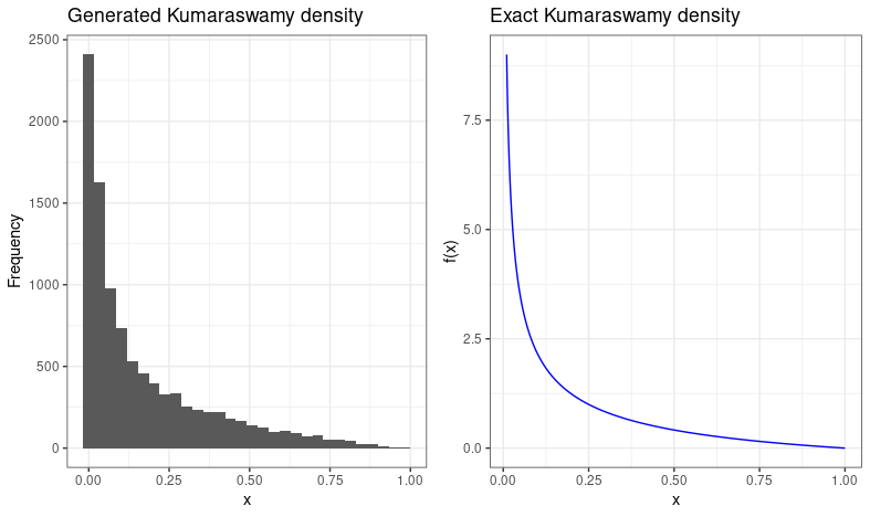
Which looks pretty good :)
Cauchy distribution
We'll be a bit more circumspect with the commentary from now on. Here, we're solving for the inverse CDF of the Cauchy distribution:
$$ \begin{aligned} u &= F_X = \frac{1}{2} + \frac{1}{\pi} \arctan(\frac{(x-\mu)}{\sigma}). \\ &\implies u - \frac{1}{2} = \frac{1}{\pi} \arctan(\frac{(x-\mu)}{\sigma}). \\ &\implies \pi(u - \frac{1}{2}) =\arctan(\frac{(x-\mu)}{\sigma}). \\ &\implies \tan(\pi(u - \frac{1}{2})) = \frac{(x-\mu)}{\sigma}. \\ &\implies \sigma \tan(\pi(u - \frac{1}{2})) = x-\mu. \\ &\implies x = F_X^{-1} = \sigma \tan(\pi(u - \frac{1}{2})) + \mu. \end{aligned} $$
Here's a slightly different example of implementing the inverse-transform method; we define a more generalisable function, allowing us to specify a couple of distribution parameters. Apart from that, the idea is much the same:
# function to implement inverse-transform method, i.e,
# takes a random uniform variable, outputs a random
# variable from the Cauchy distribution with sigma
# and mu parameters.
inverse_cauchy <- function(u, sigma, mu) {
    sigma * tan(pi * (u - (1/2))) + mu
}

# generate 10000 random uniforms
unifs <- runif(10000)

# set distribution parameters
sigma <- 1 # scale
mu <- 0 # location

# generate random variables
xsim <- sapply(unifs, inverse_cauchy, sigma = sigma, mu = mu)
Again, it's a good idea to check that what we've done is actually correct. We can use the base R function rcauchy to generate from this distribution, and plot histograms alongside one another:
# use base R to generate the same values!
set.seed(1)
rcauchy_vals <- rcauchy(10000, location = 0, scale = 1)

tibble(`Inverse-transform-generated` = xsim, `Base-R generated` = rcauchy_vals) %>%
    pivot_longer(everything(), names_to = "method") %>%
    ggplot(aes(value)) +
        geom_histogram(bins = 50) +
        scale_x_continuous(limits = c(-25, 25)) +
        facet_wrap(~ method) +
        theme_bw() +
        labs(x = "x", y = "Frequency")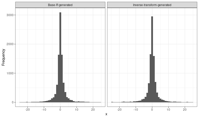
Side note: I'm not actually sure what method the base R functions use...
Weibull distribution
Even less verbose, now:
$$ \begin{aligned} F_X(x) &= u =1-\exp(\frac{x}{\lambda})^k \text{ , where x } \geq 0. \\ &\implies \log(1 - u) = (\frac{x}{\lambda})^k. \\ &\implies \log(1 - u) = \frac{x^k}{\lambda^k}. \\ &\implies \log(1 - u) \lambda^k = x^k. \\ F_X^{-1} &= x = (\log(1 - u) \lambda^k )^{1/k} \\ &= \log(1 - u)^{1/k} . (\lambda^k)^{1/k} \\ &= \lambda \log(1 - u)^{1/k}. \\ \end{aligned} $$Another way to check that we've solved for the inverse CDF correctly is to use the base R quantile functions. These are the ones that start with q. For example:
inverse_weibull_cdf <- function(u, lambda, k) {
    lambda * -log(1 - u)^(1 / k)
}

inverse_weibull_cdf(.5, 1, 1)
# [1] 0.6931472
qweibull(.5, 1, 1)
# [1] 0.6931472
Sampling from a discrete distribution
Sampling from discrete distributions is a little different than sampling from continuous distributions. Imagine we have this PDF, which tells us that \(x\) can only take on integer values from \(-2\) to \(2\):
$$ f(x) = \begin{cases} 0.20 \text{ if } x = -2, \\ 0.15 \text{ if } x = -1, \\ 0.20 \text{ if } x = 0, \\ 0.35 \text{ if } x = 1, \\ 0.10 \text{ if } x = 2, \\ 0 \text{ otherwise.} \end{cases} $$
Remember that the CDF of a random variable \(X\) evaluated at \(x\), \(F_X(x)\), is the probability that \(X \leq x\). It's therefore just a cumulative sum of the probability mass function (PMF, like the PDF but for discrete distributions) evaluated at each discrete value of \(X \leq x\); we could work this out by hand, or just use cumsum in R:
# possible x-values
x <- -2:2

# probability mass function evaluated at each x-value
fx <- c(0.20, 0.15, 0.20, 0.35, 0.10)

# evaluate the CDF at each x-value
(Fx <- cumsum(fx))
# [1] 0.20 0.35 0.55 0.90 1.00
Easy. Our CDF, therefore, is this:
$$ F_X(x) = \begin{cases} 0.20 \text{ if } x = -2, \\ 0.35 \text{ if } x = -1, \\ 0.55 \text{ if } x = 0, \\ 0.90 \text{ if } x = 1, \\ 1.00 \text{ if } x = 2, \\ 0 \text{ otherwise.} \end{cases} $$
Now, instead of finding the inverse CDF, we use the CDF directly. We still generate random uniform variables, but this time, we find the smallest value of \(X\) such that \(F(x) \geq u\):
- Step 1: Generate \(u\) from uniform(0, 1);
- Step 2: Find the smallest value of \(X\) such that \(F(x) \geq u\): That is, using the example above,
- if \(u \leq 0.20\), set \(X = -2\);
- else if \(0.20 < u \leq 0.35\), set \(X = -1\);
- ...
- else set \(X = 2\).
Okay, let's draw ten random samples from the distribution. Here's how we can implement it (keeping in mind we've already defined the CDF above, as the vector Fx):
# generate random uniforms
set.seed(1)
u <- runif(10)

# specify possible x-values
x <- -2:2

# find smallest value of x with CDF >= u, i.e., implement method
xsim <- sapply(u, function(uval) min(x[Fx >= uval]))

# render table showing u with the corresponding values of x obtained using the CDF
knitr::kable(tibble(u = u, xsim = xsim))| Simulated values | |
|---|---|
And that's all my brain can handle at this point.